Definition: A stationary time series is a time series where the statistical properties (mean, variance, autocorrelation structure, etc.) remain constant over time. In essence, it lacks trends, seasonality, or other systematic shifts in its pattern.
No Systematic Trends: Think of it as your data hovering around a roughly constant average value over time. No clear upward or downward drifts.
Variance is Consistent: Your data doesn’t get systematically more ‘spread out’ as time goes on.
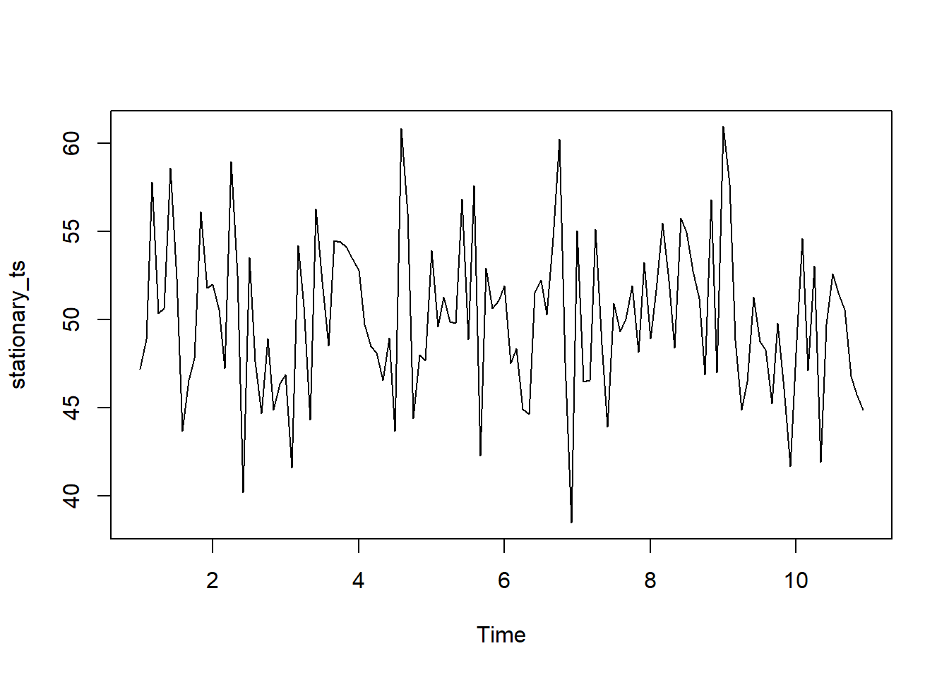
Visual Intuition: A stationary time series tends to oscillate around a constant mean with a relatively consistent amplitude of fluctuations.
Why It Matters: Lots of time series analysis methods, including ARIMA modeling, often perform best when your data is stationary (or you’ve made transformations to achieve this).
The R code below shows a time series with a constant mean and variance (i.e. stationary time series).
Reveal the Secret Within
# Generate a Stationary Time Series# Ensure your results are reproducibleset.seed(123) # Simulate 120 data pointsstationary_ts <-ts(rnorm(120, mean =50, sd =5), frequency =12) # Create a tsibble for itstationary_df <- tsibble::as_tsibble(stationary_ts)stationary_df <- dplyr::mutate(stationary_df, t = dplyr::row_number())# Normally distributed, mean of 50, variance of 25 plot(stationary_ts) # Visualize the series
1.0.1 Autocorrelation and Partial Autocorrelation Function
This section is for generating Autocorrelation Function (ACF) and Partial Autocorrelation Function (PACF) plots of the time series data. The function acf2 is used here.
No Systematic Trends: Think of it as your data hovering around a roughly constant average value over time. No clear upward or downward drifts.
Variance is Consistent: Your data doesn’t get systematically more ‘spread out’ as time goes on.
Why It Matters: Lots of time series analysis methods, including ARIMA modeling, often perform best when your data is stationary (or you’ve made transformations to achieve this).
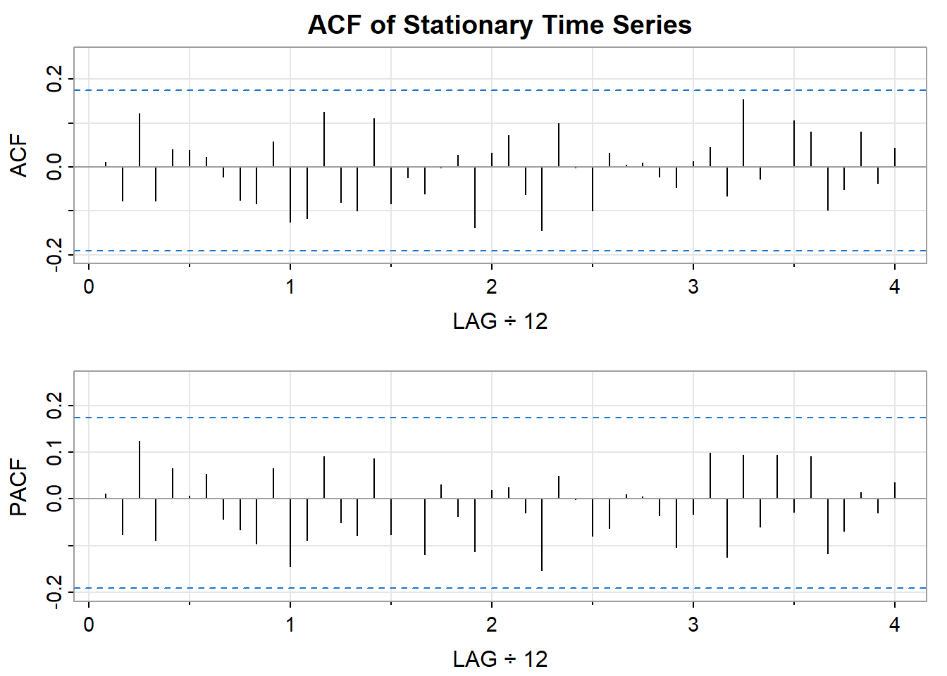
Let’s take a look at the ACF and PACF plots of this series in order to identify the best model for this series.
Reveal the Secret Within
# ACF plot for Stationary Time Series
acf_stationary <- astsa::acf2(stationary_ts, main="ACF of Stationary Time Series")
Interpreting the ACF Plot (acf_stationary)
Significant Spikes: Are there tall bars exceeding the blue dashed lines early on? This implies correlation at specific lags (e.g., today is similar to yesterday).
Decaying Pattern: Does the spike height drop rapidly, with most bars within the dashed lines after a few lags? This is common for stationary series, as further ‘echoes’ in time get fainter.
No Obvious Seasonality: If data had monthly cycles, your ACF would reflect it with repeated spikes every 12 lags. You likely won’t see this here.
What about the PACF?
The PACF would likely not show many major spikes beyond the first couple. That tells us, once you account for very short-term correlation, your ‘echoes’ mostly disappear!
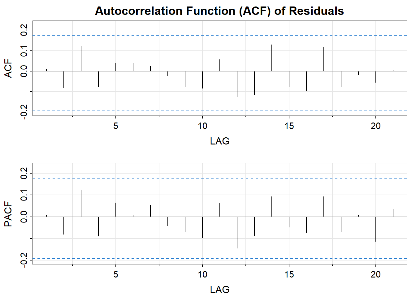
1.0.2 Statistical Tests for Autocorrelation
Other common methods is to use the Box-Ljung test or the Durbin-Watson test. These tests are used to null hypothesis that there is no autocorrelation in the data. If the p-value of the test is less than a certain significance level (e.g., 0.05), then we can reject the null hypothesis and conclude that there is autocorrelation in the data.
Durbin-Watson Test (dwtest): A formal statistical test to detect if there’s significant autocorrelation in the residuals.
Ljung-Box Test (Box.test): The Ljung-Box test checks for autocorrelation in the residuals of a time series model. Autocorrelation here means that the residuals (errors) of the model are correlated with each other at different lags.
Null Hypothesis:
H0: The data are independently distributed (i.e. the correlations in the population from which the sample is taken are 0, so that any observed correlations in the data result from randomness of the sampling process).
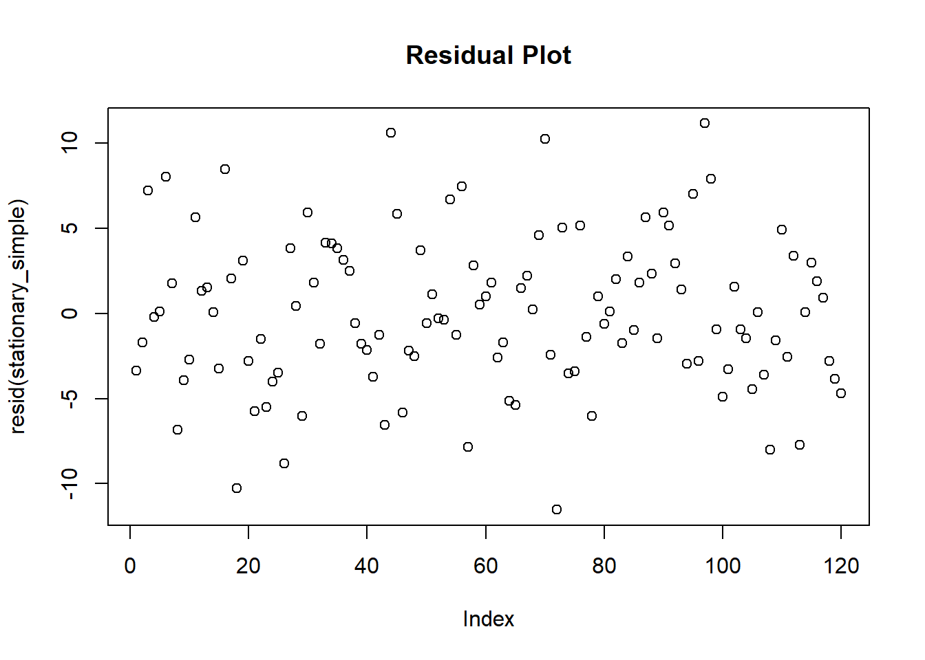
Here are some steps you can take to check for autocorrelation in your time series data:
Fit a linear regression model to your data.
Reveal the Secret Within
# Simple Linear Regression Model
stationary_simple <- stats::lm(value ~ t, data = stationary_df)
# View Model Summary
summary(stationary_simple)
Call:
stats::lm(formula = value ~ t, data = stationary_df)

Residuals:
     Min       1Q   Median       3Q      Max
-11.5272  -2.8354  -0.2433   2.9391  11.1638

Coefficients:
             Estimate Std. Error t value            Pr(>|t|)
(Intercept) 50.581625   0.823364  61.433 <0.0000000000000002 ***
t           -0.008337   0.011810  -0.706               0.482
---
Signif. codes:  0 '***' 0.001 '**' 0.01 '*' 0.05 '.' 0.1 ' ' 1

Residual standard error: 4.482 on 118 degrees of freedom
Multiple R-squared:  0.004206,  Adjusted R-squared:  -0.004233
F-statistic: 0.4984 on 1 and 118 DF,  p-value: 0.4816
## Durbin-Watson Test
lmtest::dwtest(stationary_df$value ~ stationary_df$t)
    Durbin-Watson test

data:  stationary_df$value ~ stationary_df$t
DW = 1.9701, p-value = 0.3979
alternative hypothesis: true autocorrelation is greater than 0
Perform a Box-Ljung test on the residuals.
Reveal the Secret Within
# Box-Ljung test Box.test(stationary_simple$residuals, lag =24, type ="Ljung-Box")
# Stationary Time Series```{r libraries-1,message = FALSE,warning=FALSE, echo=FALSE}# Load necessary libraries# tsibble: A 'Tidy' Time Series Data Structure# Provides an organized framework for manipulating, storing, and working with time series data in R.pacman::p_load(tsibble) # feasts: Feature Extraction and Statistics for Time Series # Offers specialized functions for extracting valuable features (e.g., trend, seasonality) from time series data and facilitates statistical analysis of these features.pacman::p_load(feasts)# fable: Forecasting Models for Tidy Time Series# Contains flexible methods and tools for developing forecasting models, specifically tailored to work with time series data represented in the tsibble structure.pacman::p_load(fable)# astsa: for Applied Statistical Time Series Analysis# Provides functions and datasets specifically geared towards time series analysis and its practical applications.pacman::p_load(astsa)# lmtest: for diagnostic testing in linear regression models# Offers tools to validate assumptions of linear regression models and identify potential issues.pacman::p_load(lmtest)# forecast: for time series forecasting# Contains methods for automated forecasting techniques like exponential smoothing and ARIMA modeling.pacman::p_load(forecast)# dplyr: for data manipulation# Streamlines data transformation, filtering, and summarizing tasks with an intuitive syntax.library(dplyr)# zoo: for time series data handling# Provides features for irregular time series and specialized methods for managing such data.library(zoo)# tidyverse: an opinionated collection of R packages for data science# Includes packages like dplyr, ggplot2 for data manipulation, visualization, and other core data science tasks.pacman::p_load(tidyverse)# tidymodels: for modeling and statistical analysis# A unified framework for diverse modeling approaches, supporting consistent workflows and syntax.pacman::p_load(tidymodels)# car: for Companion to Applied Regression# Provides datasets and functions focused on regression analysis, with emphasis on diagnostics and visualization.pacman::p_load(car)# stats: for statistical functions in R (usually loaded by default)# Offers a fundamental set of statistical tools for modeling, analysis, and testing.pacman::p_load(stats)# extraDistr: extends the range of statistical distributions available# Adds a variety of distributions beyond those in the base R installation for more nuanced modeling or simulations.pacman::p_load(extraDistr)# ggplot2: A 'ggplot2' extension that enables the rendering of complex formatted plot labels (titles, subtitles, facet labels, axis labels, etc.). Text boxes with automatic word wrap are also supported.pacman::p_load(ggplot2)# ggtext: Rich Text Formatting for 'ggplot2' Graphics# Extends the graphical capabilities of 'ggplot2' by allowing you to use complex HTML and Markdown-like formatting styles within plot elements (titles, labels, captions, annotations, etc.). pacman::p_load(ggtext)# patchwork: Combine 'ggplot2' Plots # Streamlines arrangement of multiple 'ggplot2' (or related) plots into a single layout for clear and concise visualizations.library(patchwork) # gridExtra: Functions in Grid Graphics# Facilitates arrangement and customization of multiple ggplot2 (or other grid-based) plots in a single layout.pacman::p_load(gridExtra)# Set random seed for reproducibility of resultsset.seed(123) options(scipen = 999)```**What is a Stationary Time Series?**- **Definition:** A stationary time series is a time series where the statistical properties (mean, variance, autocorrelation structure, etc.) remain constant over time. In essence, it lacks trends, seasonality, or other systematic shifts in its pattern. - **No Systematic Trends:** Think of it as your data hovering around a roughly constant average value over time. No clear upward or downward drifts. - **Variance is Consistent:** Your data doesn't get systematically more 'spread out' as time goes on.- **Visual Intuition:** A stationary time series tends to oscillate around a constant mean with a relatively consistent amplitude of fluctuations.- **Why It Matters:** Lots of time series analysis methods, including ARIMA modeling, often perform best when your data is stationary (or you've made transformations to achieve this).The R code below shows a time series with a constant mean and variance (i.e. stationary time series).```{r stationary-1,error = FALSE,message = FALSE,warning=FALSE}# Generate a Stationary Time Series# Ensure your results are reproducibleset.seed(123) # Simulate 120 data pointsstationary_ts <- ts(rnorm(120, mean = 50, sd = 5), frequency = 12) # Create a tsibble for itstationary_df <- tsibble::as_tsibble(stationary_ts)stationary_df <- dplyr::mutate(stationary_df, t = dplyr::row_number())# Normally distributed, mean of 50, variance of 25 plot(stationary_ts) # Visualize the series ```### Autocorrelation and Partial Autocorrelation FunctionThis section is for generating Autocorrelation Function (ACF) and Partial Autocorrelation Function (PACF) plots of the time series data. The function **`acf2`** is used here.- **No Systematic Trends:** Think of it as your data hovering around a roughly constant average value over time. No clear upward or downward drifts.- **Variance is Consistent:** Your data doesn't get systematically more 'spread out' as time goes on.- **Why It Matters:** Lots of time series analysis methods, including ARIMA modeling, often perform best when your data is stationary (or you've made transformations to achieve this).Let's take a look at the ACF and PACF plots of this series in order to identify the best model for this series.```{r stationary-acf,message = FALSE,error = FALSE,warning=FALSE}# ACF plot for Stationary Time Series acf_stationary <- astsa::acf2(stationary_ts, main="ACF of Stationary Time Series") ```**Interpreting the ACF Plot (`acf_stationary`)**1. **Significant Spikes:** Are there tall bars exceeding the blue dashed lines early on? This implies correlation at specific lags (e.g., today is similar to yesterday).2. **Decaying Pattern**: Does the spike height drop rapidly, with most bars within the dashed lines after a few lags? This is common for stationary series, as further 'echoes' in time get fainter.3. **No Obvious Seasonality:** If data had monthly cycles, your ACF would reflect it with repeated spikes every 12 lags. You likely won't see this here.**What about the PACF?**- The PACF would likely not show many major spikes beyond the first couple. That tells us, once you account for very short-term correlation, your 'echoes' mostly disappear!### Statistical Tests for AutocorrelationOther common methods is to use the Box-Ljung test or the Durbin-Watson test. These tests are used to null hypothesis that there is no autocorrelation in the data. If the p-value of the test is less than a certain significance level (e.g., 0.05), then we can reject the null hypothesis and conclude that there is autocorrelation in the data.- **Durbin-Watson Test (`dwtest`):** A formal statistical test to detect if there's significant autocorrelation in the residuals.- **Ljung-Box Test `(Box.test)`:** The Ljung-Box test checks for autocorrelation in the residuals of a time series model. Autocorrelation here means that the residuals (errors) of the model are correlated with each other at different lags.**Null Hypothesis:**- H0: The data are independently distributed (i.e. the correlations in the population from which the sample is taken are 0, so that any observed correlations in the data result from randomness of the sampling process).Here are some steps you can take to check for autocorrelation in your time series data:1. Fit a linear regression model to your data.```{r stationary-lm, message = FALSE,warning=FALSE, error=FALSE} # Simple Linear Regression Model stationary_simple <- stats::lm(value ~ t, data = stationary_df) # View Model Summary summary(stationary_simple) ```2. Calculate the residuals from the model.```{r stationary-residuals, warning=FALSE, error=FALSE} stationary_simple_residuals <- resid(stationary_simple) ## Visual Check for Patterns plot(resid(stationary_simple)) + title(main = "Residual Plot") ```3. Plot the autocorrelation function (ACF) of the residuals.```{r residuals-acf-1, message = FALSE,warning=FALSE, error=FALSE} ## Autocorrelation Check astsa::acf2(resid(stationary_simple), main= paste0("Autocorrelation Function (ACF) of Residuals")) ```4. Perform a Durbin-Watson test on the residuals.```{r DurbinWatson-1, warning=FALSE, error=FALSE, message=FALSE}## Durbin-Watson Test lmtest::dwtest(stationary_df$value ~ stationary_df$t)```5. Perform a Box-Ljung test on the residuals.```{r BoxLjung-1, warning=FALSE, error=FALSE, message=FALSE}# Box-Ljung test Box.test(stationary_simple$residuals, lag = 24, type = "Ljung-Box")```